Clay Lenhart’s Blog

This is a second entry in a series on SQL Server Analysis Services (SSAS). To see the other blog entries on this tutorial, click on the SSAS Beginner’s Guide on the top bar.

Relational Databases

Let’s take a quick look at a relational database table of football players:

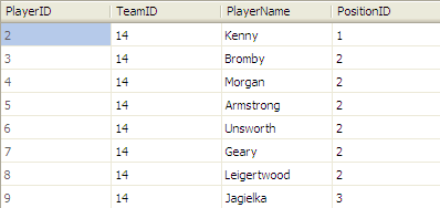
The table is structured in rows and columns. Note that the column names are fixed – they are not based on the data. This is a difference between relational databases and SSAS databases.

SSAS databases are typically loaded from the relational database to the SSAS database and a copy of the data stored in a different form in the SSAS database. Once the data has been copied, you can delete the relational database (This assumes you are using the default MOLAP option).

2 Dimensional SSAS Databases

SSAS databases are stored in multidimensional structures. Below is an example of an SSAS database with just 2 dimensions. This contains fantasy football points, so the “2” in the first row and first column is the fantasy football points that Reina received during the 11/Aug/2007 game week.

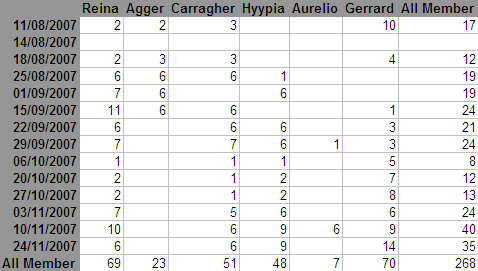
The grey area contains two dimensions: Players and Game Weeks. Each column header (and row label) is called a dimension member. Example dimension members are “Carragher” and “03/11/2007″. These dimension members are similar to column names, however they are based on data.

Each number in a cell is at the intersection of two dimension members. Take for instance Gerrard’s first match where he received 10 points. It is stored at the intersection of

• “Gerrard”
• and “11/08/2007″

Gerrard and “11/08/2007″ are coordinates to the cell containing 10. When you start writing MDX queries, you will try to find ways to reference these cells using coordinates.

The All Member aggregation is what is really useful in SSAS databases. It is a member that is added to each dimension when loading the data. The All Member cells are pre-calculated when loading the SSAS database data and are typically a sum. This member is physically stored and you can also query All Members just like any other member. The All Member aggregation above makes it easy to answer questions like, “What is the total number of points that Gerrard received?” The answer is found at the intersection of

• “Gerrard”
• And the Game Week’s “All Member”.

You can reference the All Members using the coordinate system just like any other member of the dimension.

3 Dimensional SSAS Database

Let’s take a look at a 3 dimensional SSAS database:

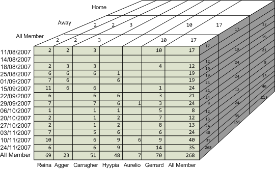
The diagram above shows most of the values stored in the 3 dimensional SSAS database. There are some values in the back of the cube that you can’t see without cutting the cube open, but they still exist.

The cube is shown so that the front pane is the same data as the two dimensional SSAS database above.

Just as a side note, although the diagram has two 10s on the cell for Gerrard on 11/08/2007, on the front in grey and on the top of the cell in white, the cell block itself only contains the number once. The cells can only contain one number and the numbers shown are for the 3D block, rather than a 2D pane. So the cell contains just 17, even though 17 is shown three times.

The only difference with 3D cubes is that locating a cell requires 3 coordinates instead of 2:

• Game week
• Player
• Home/Away

The 3^rd dimension, Home/Away, gives us more information about the scores compared to the 2 dimensional database. If you wanted to know how many points these players received for all Away matches, you would go to the intersection of these three coordinates:

• Game week’s “All Member”
• Player’s “All Member”
• and Home/Away’s “Away” member

Here you will find the value “155”.

The cube can answer other questions. Although you cannot see it in the diagram, the cube stores total points that Gerrard received at home. You would find it at the intersection of

• the game week’s “All Member”
• “Gerrard”
• “Home”.

This value would be found on the bottom plane just to the left of the value 155.

4 or More Dimensions

There is really no limit to the number of dimensions you can create in your database even though it might be difficult to visualize. Let’s say you want to track sales for the following:

• the year 2007
• the southeast region
• the product “gizmo”
• and the “Acme” store

You may not be able to see how all the data is stored, however this scenario does have 4 dimensions.

I am going to use this blog to convince a friend to use SQL Server Analysis Services (SSAS) in his projects because it makes it easier to write reports on as compared to relational databases. Part of the challenge is that people don’t realize its advantages, and part is the large learning curve to use it.

This first post is on it advantages. Next will be a whole series to make it a bit easier to learn. First there are two main advantages for using SSAS.

You might have been attracted to article marketing because it enables you to take part in effectively advertising your site online via articles that you make and submit to internet publishers. Article marketing has a lot of facets and unique heights of skills to learn, but it’s doable and understandable to the majority of website owners, even ones who do not own a background in SEO (search engine optimization). Look through this page for details on personal alarm safety.

SSAS is fast even on a large volume of data

Well, as long as the queries return few rows, and this really gets at the heart of when you want to use SSAS and when you don’t. It is good at returning a single sum for a column over a large number of rows, but is very slow at returning a lot of detailed rows. The reason for this is the totals (and the subtotals) are stored in the SSAS database. It takes more work to read all the original rows than the one single subtotal value. In fact, relational databases will be faster at returning detailed rows compared to SSAS.

Take for example the following SQL code from a relational database:

SELECT SUM(Cost)FROM Sales

In SQL Server, this query could take a very long time as it scans the Sales table, however in SSAS the result comes back instantly because the one value is already pre-calculated and stored in the SSAS database.

SSAS’s calculated measures are fast execution-wise and easy reusable

In relational databases, calculation code can get messy. The main problem with SQL SELECT statements is that they make it difficult to write a calculation once, like in a function, and GROUP BY different ways. You might build a SELECT statement in a string and execute the string using sp_executesql, or you use a CASE statement to list the different SELECT statements that group differently. Both are messy compared to SSAS.

Calculated measures in SSAS give you a way to define the calculations in a straight forward manner that does not matter how you will group the data later. They also you another advantage in that they are defined centrally in the SSAS database, and the reports pick and choose the calculated measures they want. This moves formulas from many reports to the central SSAS database where they are tested once.

Between having one set of centralized “official” formulas, and having formulas written in clear straight forward manner, the reports will have fewer number of bugs.